From Points to Physics
Building the mathematics of a graphics pipeline

04
Year — 2025
Categories
Role
- MSc coursework — University of Edinburgh
- Individual implementation — C++, Eigen, Polyscope
- Five assessed reports: geometry, simulation, debugging
CGGS — Computer Graphics: Geometry and Simulation
A graphics pipeline is only as honest as the mathematics underneath it. This course asked for that mathematics to be written from scratch in C++: fitting surfaces to raw point clouds, measuring how a mesh bends, flattening it onto a plane without tearing it, and pushing rigid and deformable bodies through a stable time step. Five assessed reports — and a closing one that was pure forensics: six defects found by reading the maths, not the stack trace.
Problem
Geometry processing rests on a stack of small, unforgiving linear algebra problems. A point cloud carries no surface — only samples and normals. A triangle mesh carries no curvature — only positions and connectivity. A simulator does not know, unless told, that a rotation is not a strain. Each of those gaps is closed by one specific discrete operator, and a single wrong sign or transposed product produces output that still renders, still animates, and is still wrong.
The brief was to build those operators directly against Eigen and Polyscope, then argue from the results rather than from the textbook: which formulation, at which parameters, and at what cost.
Reconstruction
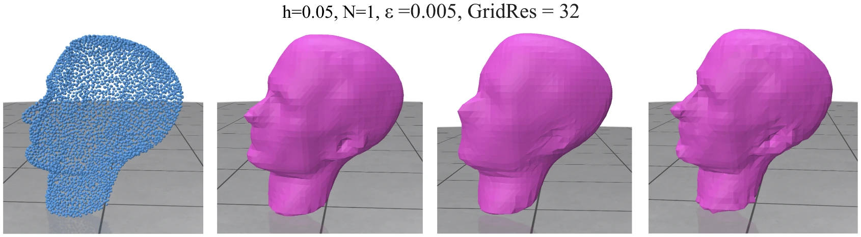
The first surface came from scalar polynomial moving least squares. Around every node of a voxel grid a trivariate polynomial of degree N is fitted to the nearby samples by weighted least squares, with off-surface constraints displaced along each normal to pin the sign of the implicit function and a local SVD solve for the coefficients. Where a cell holds fewer neighbours than the polynomial has coefficients the system is underdetermined, so the node is marked NaN rather than guessed. The zero level set of the resulting field is what gets meshed.
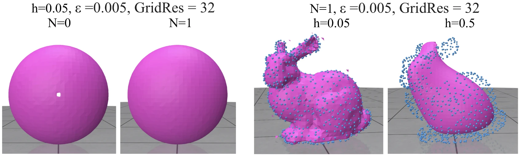
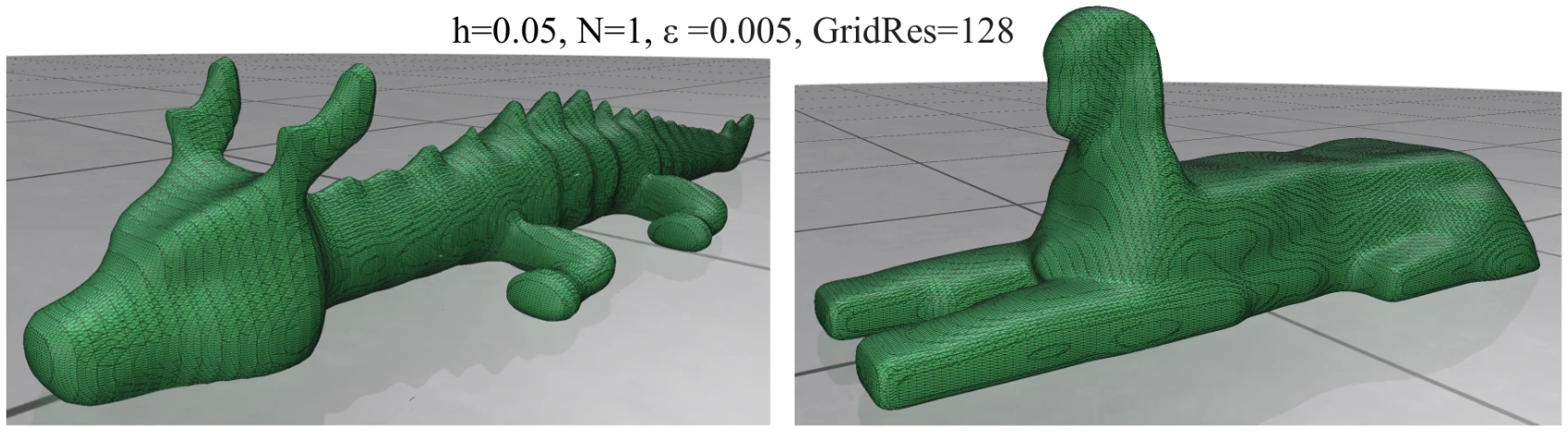
The weight kernel sets the character of the surface. Wendland support falls smoothly to zero at radius h and gave the most stable result; a Gaussian never quite vanishes, so distant points keep voting and detail blurs; a singular kernel weights the nearest samples hardest, sharpening edges and surfacing subtle local structure. Degree and support behave as a pair — at N = 0 a hole opens in the sphere that N = 1 closes, and lifting h from 0.05 to 0.5 trades the bunny’s ears for a smooth blob.
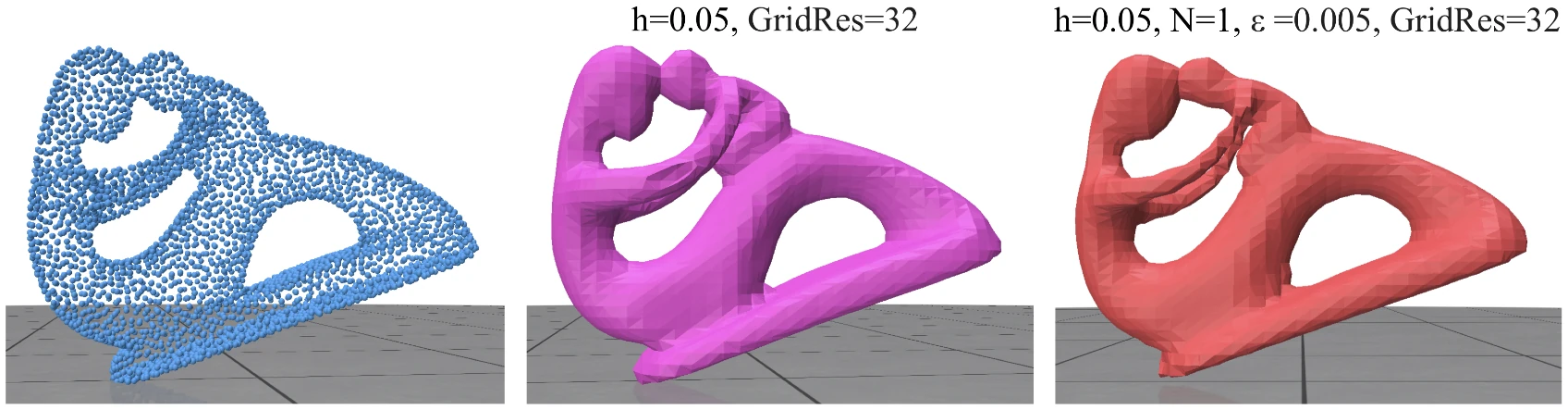
A second formulation skipped the per-node solve entirely. Function-blending MLS defines one distance function per point and blends them through Wendland weights as a partition of unity, so each grid location simply looks up its neighbours, dots each normal, and averages. No offset points, no linear system — and the same shape in 46.8 seconds against 92.6 for the polynomial fit.
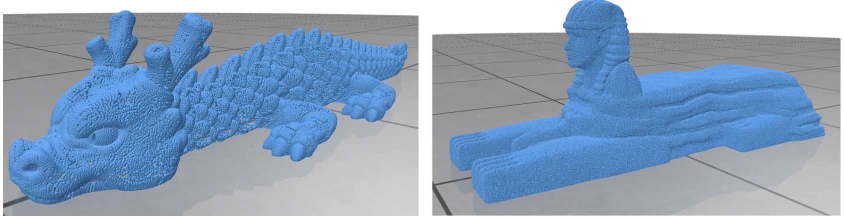
A double loop over every point for every grid cell is O(N·G). At 257,087 points and 128³ cells, the algorithm stops being slow and starts being impractical.
Scale
The fix was a spatial index. The preprocessed on- and off-surface points are loaded once into a k-d tree — recursive median splits along alternating coordinate axes — so each grid node asks only for the samples inside radius h instead of scanning the entire cloud. A query descends only into subtrees that could contain a hit, taking the typical lookup to logarithmic cost and the per-cell work down to a bounded neighbourhood.
That made a 128³ reconstruction of both models tractable, at roughly 6,977 and 6,867 seconds. The meshes came back smooth but softer than the clouds that fed them, and the report says so plainly: at h = 0.05 on a grid of 128 the support radius and the cell size are themselves a low-pass filter, and some high-frequency detail is gone before the fit even begins. The fitting mathematics is identical to the naive version — the index only changes which points it sees.
Discrete curvature
The second geometry report moved from building surfaces to measuring them. Gaussian curvature falls out of the angle defect — how far the angles meeting at a vertex fall short of a full turn — normalised by that vertex’s Voronoi area. Mean curvature comes from the cotangent-weighted Laplacian, whose action on vertex positions returns the mean curvature normal. Both were assembled from the ground up: face angles, then area distribution, then the operator.
The maps behaved as theory predicts. Saddle regions read negative and bulges positive, ridges and flats separated cleanly, and the noisier patches landed exactly where the triangulation is least regular — which is itself the useful result, because it shows the estimator degrading with mesh quality rather than with shape.
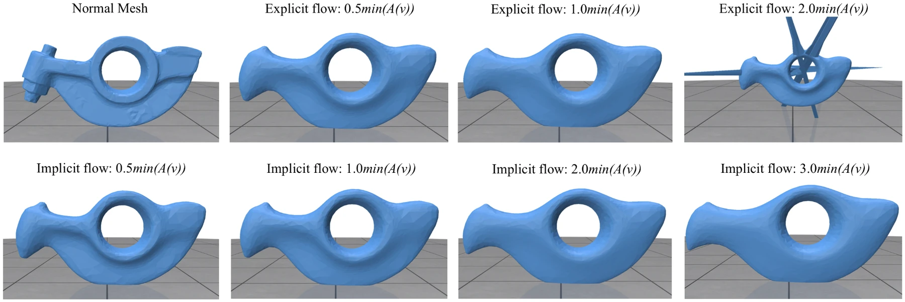
Mean curvature flow then moves every vertex along that normal. The explicit step is one matrix–vector product and is only conditionally stable: at 0.5 and 1.0 times the smallest vertex area the rocker arm smooths gradually, and at 2.0 it detonates into spines. The implicit step solves a linear system for the new positions instead and stayed stable out to 3.0 — the same five seconds of flow, far more of it actually delivered.

Flattening
Mapping a surface onto the plane is where trade-offs turn sharp. Tutte’s embedding pins the boundary loop of a disc-topology mesh to a circle, spaced in proportion to edge length, then solves one harmonic system for every interior vertex — a cotangent-weighted operator built from the edge–vertex incidence matrix. It is guaranteed to produce a valid, fold-free layout. It is equally guaranteed to distort, because the circle is imposed rather than earned: on a cut bunny the checker cells stretch and shear wherever the surface curved hardest.
The second method was written from scratch. Least Squares Conformal Maps asks each triangle’s map to sit as close as possible to a similarity — the discrete form of the Cauchy–Riemann conditions — which lets the boundary find its own shape. A new lscm_parameterization header builds a local 2D frame per triangle, emits one conformality row per triangle into a large sparse system, and pins two vertices at (0,0) and (1,0) to remove the global similarity the energy cannot see.
Rather than assemble the full KKT saddle-point system, the pins were applied as heavy diagonal penalties, leaving a symmetric positive definite normal-equation system that Eigen’s SimplicialLDLT factorises directly — a deliberate simplicity-for-exactness trade, and the reasoning for it is set out in the report. Both methods were wired behind one toggle in the viewer so the two layouts could be compared on the same mesh, by eye and by distortion metric.
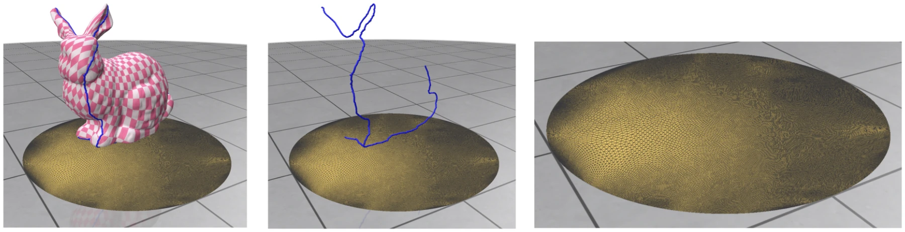
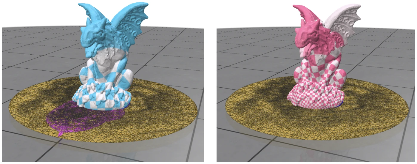
A conformal map is only fixed up to a similarity. Pin two vertices, and the rest is a sparse solve.
Rigid bodies
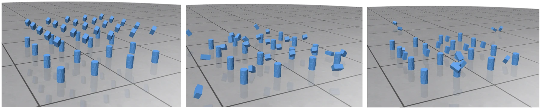
The simulation half opened with free motion and contact — a grid of cuboids dropped onto fixed cylinders. Response was clean: no interpenetration, no jitter, no popping, which says the detection and resolution logic is sound. The bodies also bounced forever, because a restitution that high with no friction or damping has nowhere to put the energy. Correct collision handling and plausible physics are not the same thing.
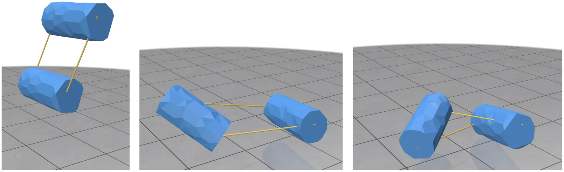
Distance constraints came next, tying vertices on one cylinder to counterparts on the other. The iterative solver held the pair together through translation and rotation, converting a free collision into a controlled knocking — and exposed its own artefacts, with constraint lines twisting unnaturally and the bodies never quite settling: the signature of position and velocity corrections competing inside the same step.
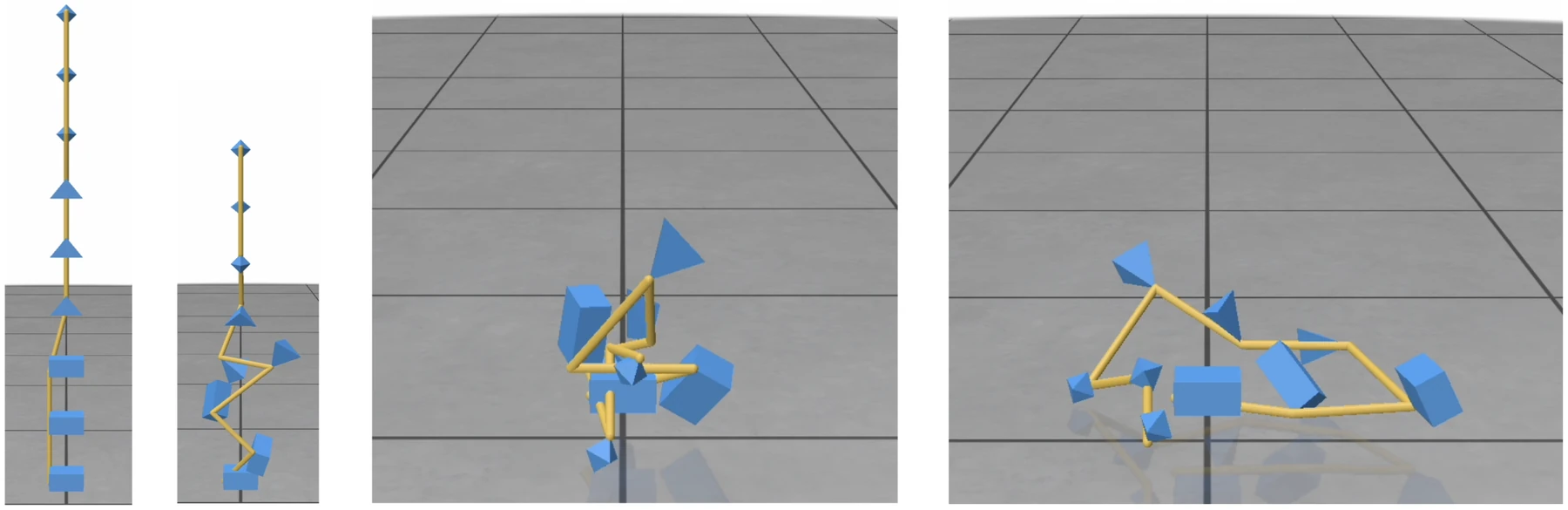
The third version was about scale. The update loop gained a broad phase — a bounding radius per mesh, so any pair whose centres of mass are further apart than the sum of their radii is rejected before narrow-phase testing — and a dirty-constraint queue that re-checks a constraint only when a mesh it touches has actually been corrected, instead of sweeping every constraint every iteration. On a tower-and-chain scene it held frame rate; on trivial scenes the bookkeeping cost more than it saved, which is the honest boundary of the optimisation and is reported as one.
Soft bodies
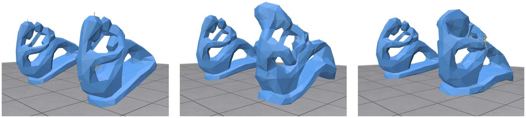
Deformable bodies ran on linear FEM under implicit integration: one velocity solve per step against a system matrix assembled from mass, damping and stiffness, then a position update from the solved velocity. Because stiffness is constant for a linear material, that matrix can be factorised once at scene initialisation and reused every step — cheap, robust, and correct for small strain. It is also wrong in a specific, visible way: linear elasticity reads a large rotation as strain, so under a strong impulse the fertility model shears and swells instead of turning.
Corotational elements fix precisely that. Each tetrahedron’s rest stiffness is computed once from the undeformed coordinates; then every step a best-fit rotation is extracted from the deformed element and its block rebuilt as R K R transpose before assembly, so pure rotation no longer registers as strain and the shearing and volume blow-up go with it. The price is structural rather than incidental: the global matrix has to be re-assembled and re-factorised on every single step, moving the dominant cost out of initialisation and into the inner loop.
Debugging
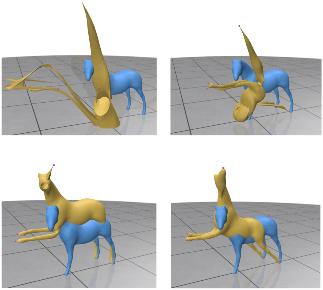
The closing report was a diagnosis exercise: two implementations that compiled, ran, and produced confident nonsense. As-rigid-as-possible deformation was returning a horse with tall spikes and collapsed limbs. Reading the output as evidence rather than noise — spikes mean the global step is under-constrained, twisting means an orientation is inverted — narrowed it to three defects: the weight matrix was missing from the right-hand side of the global solve, the edge vector was built with its endpoints subtracted in the wrong order, and the local step ran its SVD inside the per-neighbour loop with the matrix product transposed. Restoring the weights, reversing the subtraction, and lifting the SVD out of the loop with the product ordered correctly walked the mesh through four stages back to a clean, natural bend.
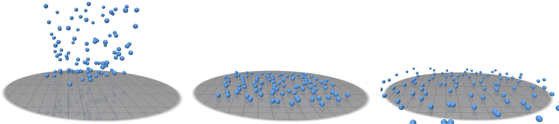
The multi-body sphere simulation failed differently — spheres sinking into each other, hanging in mid-air, and shooting off. Three more defects, each a distinct physical mismatch: a squared-distance collision test measured against twice the squared radius where the correct threshold is four times it, an inverted sign on the floor-rebound velocity check, and a gravity term switched off by a proximity conditional at exactly the moment two spheres were closest, turning attraction into separation. Replacing that conditional with a clamped denominator kept the force finite rather than absent, and the spheres began to gather, bunch, and scatter the way the model says they should.
By the numbers
- Assessed reports
- 5
- Largest cloud reconstructed
- 257,087
- Isosurface grid
- 128³
- Blended vs fitted MLS
- 46.8 s / 92.6 s
- Parameterizations built
- Tutte + LSCM
- Defects traced and fixed
- 6
Takeaway
Across five reports the same discipline kept paying: choose the discretisation, then defend it. Wendland over Gaussian because its support actually ends. Implicit over explicit because stability is worth a solve. LSCM over Tutte when angles matter more than a tidy boundary. Corotational over linear the moment the motion contains rotation. Every one of those is a cost traded for a property, and the reports argue the trade instead of asserting it.
The debugging chapter is the part that transfers furthest. Six defects, none of which crashed anything — they produced smooth, plausible, confidently wrong geometry. Finding them meant reading the shape for what it implied about the algebra, which is the skill that outlives any one codebase.
- University of Edinburgh, School of Informatics
Next case study
05 / 11